Spectral Models

Overview

sensipy supports time-resolved spectral models that describe how the source emission evolves over time. The data should contain spectra at varying times (or lightcurves at varying energies, depending on how you prefer to think about it).

Currently, the supported file formats are:

• CSV files (recommended)
• FITS files
• Text files (directory of .txt files)

Note

CSV files are the current recommended format for sensipy spectral models due to their flexibility and ease of use.

Mock Data Files

The package includes example mock data files that you can use for testing and learning. These files are installed with the package and can be accessed using the get_data_path() utility function:

• Directorydata/

  • Directorymock_data/

    • GRB_42_mock.csv (CSV format spectral model)
    • GRB_42_mock.fits (FITS format spectral model)
    • GRB_42_mock_metadata.csv (metadata for the source)

These example files demonstrate the expected format and can be used to test your setup. For real analysis, you’ll need to provide your own spectral model data.

CSV File Format

The code expects a CSV file with three columns: time, energy, and flux (dNdE) with the following units:

• time: seconds (s)
• energy: GeV
• dNdE: 1 / (cm² s GeV) - differential flux

Multiple spectra can be included in the same file, each with a different time. The code will automatically organize the data into a time-energy grid.

Sample CSV File

A full sample CSV file is included with the package. The first rows look something like this:

time [s],energy [GeV],dNdE [cm-2 s-1 GeV-1]
1.061,1.04823,1e-08
1.061,1.14937,8.3179e-09
1.061,1.26026,6.9185e-09
1.061,1.38184,5.7547e-09
1.061,1.51516,4.7861e-09
...

Column Name Flexibility

The CSV reader is flexible with column names:

• Column names are case-insensitive
• Substring matching is supported (e.g., “Time” will match “time [s]”)
• The code looks for columns containing: time, energy, and flux or dnde

Loading a CSV File

from sensipy.source import Source
from sensipy.util import get_data_path
import astropy.units as u

# Get path to package mock data
mock_data_path = get_data_path("mock_data/GRB_42_mock.csv")

# Load CSV spectral model
source = Source(
    filepath=str(mock_data_path),
    min_energy=30 * u.GeV,
    max_energy=10 * u.TeV,
)

# Optionally add EBL absorption
source_with_ebl = Source(
    filepath=str(mock_data_path),
    min_energy=30 * u.GeV,
    max_energy=10 * u.TeV,
    ebl="franceschini"
    z=0.5,
)

FITS File Format

FITS files can also be used to store spectral models. The expected structure is:

• HDU[1]: Energy array (in GeV)
• HDU[2]: Time array (in seconds)
• HDU[3]: Flux array (2D, shape: [n_energy, n_time], units: cm⁻² s⁻¹ GeV⁻¹)
• HDU[0] (optional): Metadata (source properties)

FITS Example

from sensipy.source import Source
from sensipy.util import get_data_path
import astropy.units as u

# Get path to package mock data
mock_fits_path = get_data_path("mock_data/GRB_42_mock.fits")

# Load FITS spectral model
source = Source(
    filepath=str(mock_fits_path),
    min_energy=30 * u.GeV,
    max_energy=10 * u.TeV,
    ebl="dominguez",
    z=0.5,
)

Metadata

Metadata provides additional information about the source, such as sky coordinates, distance, energy output, and jet properties.

User-Defined Metadata

sensipy uses a completely user-defined metadata system. There are no built-in metadata fields—you define whatever metadata keys you need for your analysis. Metadata is stored in a dictionary and can be accessed via attribute notation (similar to pandas DataFrame columns).

CSV Metadata File

For CSV spectral models, you can provide a separate metadata file with the same basename plus _metadata.csv:

GRB_42_mock.csv
GRB_42_mock_metadata.csv

The metadata CSV file should have columns: parameter, value, and optionally units:

parameter,value,units
event_id,42.0,
longitude,0.0,rad
latitude,1.0,rad
distance,100000.0,kpc

Any parameter names you include will be stored in the metadata dictionary. The units column is optional—if provided, values will be converted to astropy Quantity objects with the specified units.

FITS Metadata

For FITS files, metadata can be included in the header of HDU[0] using a flexible format. sensipy reads any non-standard FITS header keys and converts them to metadata.

FITS Header Format

The FITS header format uses a comment field to specify the metadata slug and optional unit:

from astropy.io import fits

header = fits.Header()
# Format: header["FITS_KEY"] = (value, "slug [unit]")
header["EVENT_ID"] = (42, "event_id")
header["LONG"] = (0.0, "longitude [rad]")
header["LAT"] = (1.0, "latitude [rad]")
header["DISTANCE"] = (100000.0, "distance [kpc]")
header["EISO"] = (2e50, "eiso [erg]")

# Empty values are ignored
header["AUTHOR"] = ("", "author")  # This will be skipped

# Keys without comments use the header key name (lowercase) as the slug
header["CUSTOM_FIELD"] = (123.45, "")  # Stored as "custom_field"

Format rules:

• Value: The actual metadata value (number or string)
• Comment: Format "slug [unit]" where:
  • slug is the metadata key name (will be converted to lowercase, spaces/special chars become underscores)
  • [unit] is optional - if provided, the value is converted to an astropy.units.Quantity or astropy.coordinates.Distance object
• Empty values: Header entries with empty string values are ignored
• No comment: If no comment is provided, the header key name (lowercase) is used as the slug

Special handling:

• Keys named distance or dist with units are converted to astropy.coordinates.Distance objects
• Standard FITS keywords (like SIMPLE, BITPIX, NAXIS, etc.) are automatically skipped

Example:

from sensipy.source import Source
from sensipy.util import get_data_path

# Load FITS file with flexible metadata
mock_fits_path = get_data_path("mock_data/GRB_42_mock.fits")
source = Source(mock_fits_path)

# Access metadata via attribute notation
print(f"Event ID: {source.event_id}")      # 42
print(f"Longitude: {source.longitude}")    # 0.0 rad
print(f"Latitude: {source.latitude}")      # 1.0 rad
print(f"Distance: {source.distance}")      # 100000.0 kpc (Distance object)

Accessing Metadata

Once loaded, metadata can be accessed in two ways:

1. Via attribute notation (recommended, similar to pandas):

from sensipy.source import Source
from sensipy.util import get_data_path

mock_data_path = get_data_path("mock_data/GRB_42_mock.csv")
source = Source(filepath=str(mock_data_path))

# Access metadata via attributes (using keys from your metadata file)
print(f"Event ID: {source.event_id}")
print(f"Distance: {source.distance}")
print(f"Coordinates: RA={source.longitude}, Dec={source.latitude}")

# Note: Only keys present in your metadata file are available
# The example above uses keys from the mock data (event_id, longitude, latitude, distance)

2. Via the metadata dictionary:

# Access the full metadata dictionary
meta = source.metadata
print(f"All metadata keys: {list(meta.keys())}")
print(f"Event ID: {meta.get('event_id')}")
print(f"Distance: {meta.get('distance')}")

Setting Custom Metadata

You can add or modify metadata at any time:

# Set custom metadata fields
source.my_custom_field = "some value"
source.another_field = 123.45

# Access them via attribute notation
print(source.my_custom_field)  # "some value"
print(source.another_field)    # 123.45

# Or via the metadata dictionary
print(source.metadata['my_custom_field'])

Note

Metadata keys are case-sensitive and must match exactly. Use the same key names that appear in your metadata file or FITS header when accessing via attributes.

Text File Directory Format

For legacy support, sensipy can also read spectral data from a directory of text files. Each file should be named with the pattern:

{basename}_tobs=NN.txt

Where NN is the observation time index. Each file contains two columns: energy (GeV) and flux (cm⁻² s⁻¹ GeV⁻¹).

Note

This format is primarily for backward compatibility. New data should use CSV or FITS formats.

Spectral Grid and Interpolation

After loading a spectral model, sensipy creates an interpolation grid in log-space (log energy, log time) to enable efficient querying at arbitrary times and energies.

Querying the Spectrum

import astropy.units as u

# Get spectrum at a specific time
time = 100 * u.s
spectrum = source.get_spectrum(time=time)

# Get flux at a specific energy and time
energy = 1 * u.TeV
flux = source.get_flux(energy=energy, time=time)

# Get lightcurve at a specific energy
lightcurve = source.get_flux(energy=energy)

The following plots demonstrate these querying methods using the mock data:

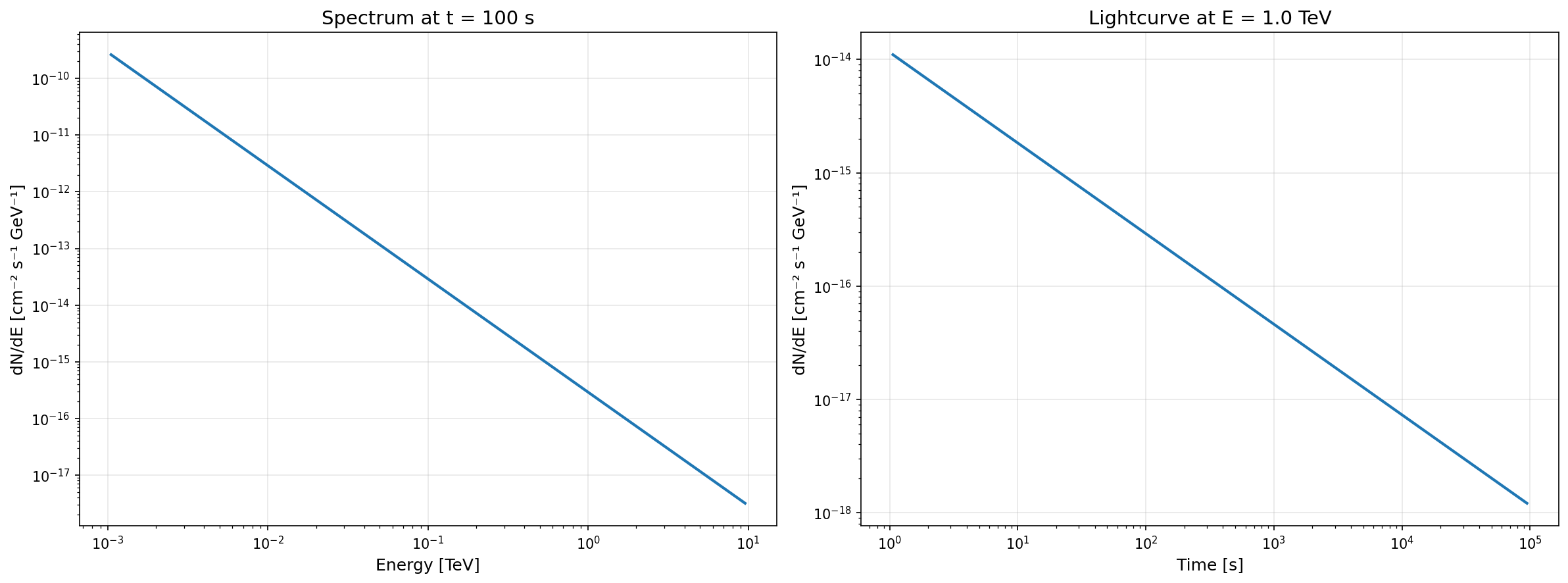
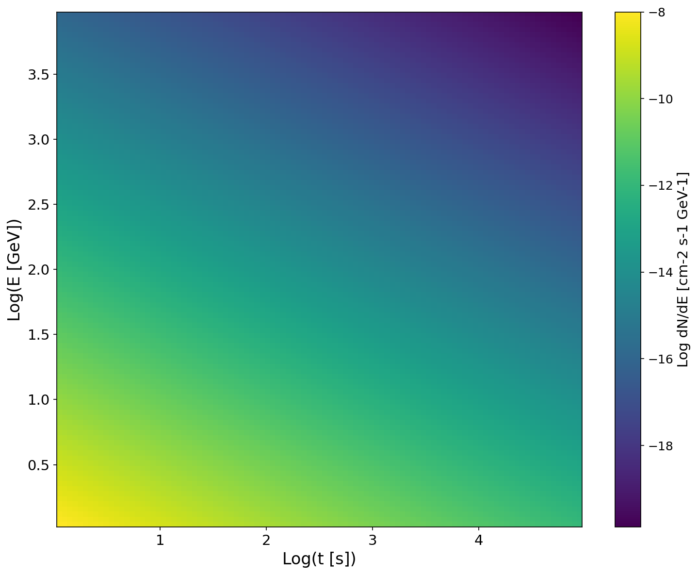
Visualizing the Spectral Pattern

The spectral pattern is a 2D plot of the spectral energy distribution (SED) as a function of time and energy.

# Show the full time-energy spectral pattern
source.show_spectral_pattern(
    resolution=100,  # Grid resolution
    return_plot=True
)

Spectral pattern visualization:

Setting Your Distance

For extragalactic sources, you need to specify the distance (or redshift) to apply EBL absorption correctly. You can set the distance either during initialization or after creating the Source object.

During Initialization

You can provide either a redshift (z) or a distance (Distance object) when creating the Source:

Using Redshift

from sensipy.source import Source
from sensipy.util import get_data_path
import astropy.units as u

mock_data_path = get_data_path("mock_data/GRB_42_mock.csv")

# Set redshift during initialization
source = Source(
    filepath=str(mock_data_path),
    min_energy=20 * u.GeV,
    max_energy=10 * u.TeV,
    z=0.5,  # Redshift
    ebl="franceschini",
)

Using Distance

from sensipy.source import Source
from sensipy.util import get_data_path
from astropy.coordinates import Distance
import astropy.units as u

mock_data_path = get_data_path("mock_data/GRB_42_mock.csv")

# Set distance during initialization
distance = Distance(3000 * u.Mpc)
source = Source(
    filepath=str(mock_data_path),
    min_energy=20 * u.GeV,
    max_energy=10 * u.TeV,
    distance=distance,  # Distance object
    ebl="franceschini",
)

Note: Only one of distance or z can be provided, not both. If both are provided, a ValueError will be raised.

After Initialization

You can also set or update the distance using the set_ebl_model() method:

Using Redshift

from sensipy.source import Source
from sensipy.util import get_data_path
import astropy.units as u

mock_data_path = get_data_path("mock_data/GRB_42_mock.csv")

# Create source without distance
source = Source(
    filepath=str(mock_data_path),
    min_energy=20 * u.GeV,
    max_energy=10 * u.TeV,
)

# Set distance and EBL model later
source.set_ebl_model("franceschini", z=0.5)

Using Distance

from sensipy.source import Source
from sensipy.util import get_data_path
from astropy.coordinates import Distance
import astropy.units as u

mock_data_path = get_data_path("mock_data/GRB_42_mock.csv")

# Create source without distance
source = Source(
    filepath=str(mock_data_path),
    min_energy=20 * u.GeV,
    max_energy=10 * u.TeV,
)

# Set distance and EBL model later
distance = Distance(3000 * u.Mpc)
source.set_ebl_model("franceschini", distance=distance)

Distance Override Priority

If you provide distance or z during initialization, it will override any distance information extracted from the metadata file. The priority order is:

1. Explicit distance or z parameter in Source() (highest priority)
2. Metadata distance from CSV or FITS file
3. No distance - EBL won’t be applied unless distance is set later

Using Your Own Data

To use your own spectral models:

1. Prepare your data in CSV or FITS format (see format details above)
2. Include metadata (optional but recommended) for source properties like distance, coordinates, etc.
3. Load the data using the Source class

from sensipy.source import Source
import astropy.units as u

# Load your custom spectral model
source = Source(
    filepath="path/to/your/model.csv",
    min_energy=30 * u.GeV,
    max_energy=10 * u.TeV,
    ebl="franceschini",  # Optional: add EBL absorption for extragalactic sources
    z=0.5,
)

Exporting to Gammapy Spectral Models

sensipy can export spectra as Gammapy spectral models for use in likelihood fitting, sensitivity calculations, and other Gammapy workflows. Two types of models are available:

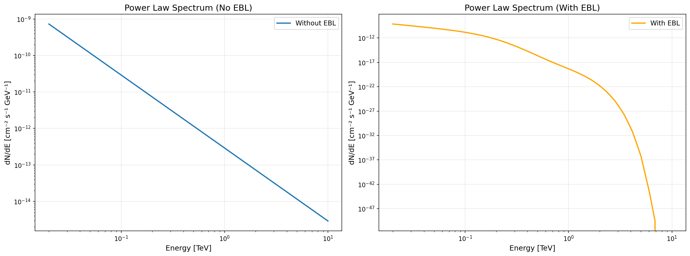
Power Law Approximation

The get_powerlaw_spectrum() method fits a power law to the spectrum at a given time and returns a PowerLawSpectralModel:

from sensipy.source import Source
from sensipy.util import get_data_path
import astropy.units as u

mock_data_path = get_data_path("mock_data/GRB_42_mock.csv")
source = Source(
    filepath=str(mock_data_path),
    min_energy=20 * u.GeV,
    max_energy=10 * u.TeV,
)

time = 100 * u.s
powerlaw_model = source.get_powerlaw_spectrum(time)

# Use in Gammapy workflows
from gammapy.modeling.models import SkyModel
sky_model = SkyModel(spectral_model=powerlaw_model)

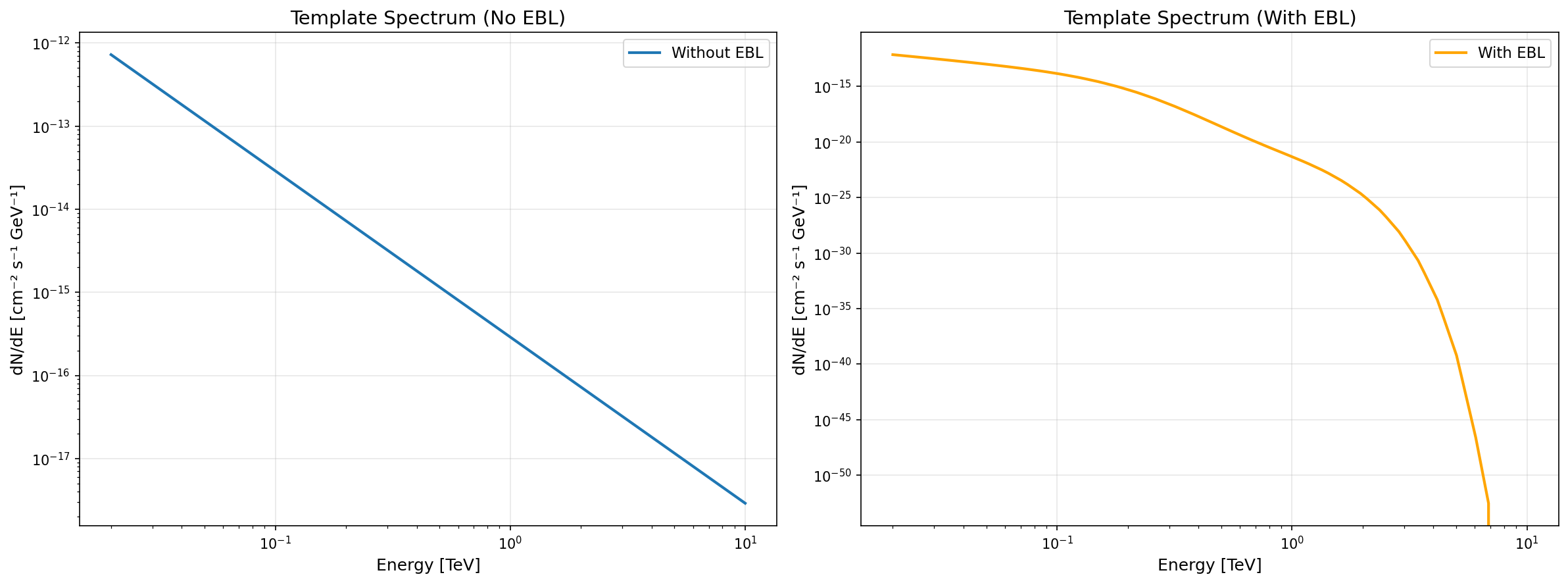
Template Spectrum

The get_template_spectrum() method extracts the full energy spectrum at a given time and returns a ScaledTemplateModel:

time = 100 * u.s
template_model = source.get_template_spectrum(time, scaling_factor=1.0)

# Template models preserve the full spectral shape
# Useful when power law approximation is insufficient

EBL Absorption

Both methods support automatic EBL absorption via the use_ebl parameter:

Power Law with EBL

source = Source(
    filepath=str(mock_data_path),
    min_energy=20 * u.GeV,
    max_energy=10 * u.TeV,
    z=1.0,
    ebl="franceschini",  # Set EBL model
)

time = 100 * u.s
# Apply EBL absorption automatically (or use default: use_ebl=None)
powerlaw_with_ebl = source.get_powerlaw_spectrum(time, use_ebl=True)

Template with EBL

source = Source(
    filepath=str(mock_data_path),
    min_energy=20 * u.GeV,
    max_energy=10 * u.TeV,
    z=1.0,
    ebl="franceschini",  # Set EBL model
)

time = 100 * u.s
# Apply EBL absorption automatically (or use default: use_ebl=None)
template_with_ebl = source.get_template_spectrum(time, use_ebl=True)

Comparison plots:

Automatic Energy Range in Plots

Both exported models have an overridden .plot() method that automatically uses the source’s min_energy and max_energy:

# Plot automatically uses source.min_energy and source.max_energy
powerlaw_model.plot()

# You can still override the energy range if needed
powerlaw_model.plot(energy_range=(0.1 * u.TeV, 5 * u.TeV))

Energy Range Considerations

When loading spectral models, you should specify the energy range of interest. This helps:

1. Optimize performance by limiting interpolation to relevant energies
2. Match observatory capabilities (e.g., CTA energy range)
3. Ensure EBL absorption is applied correctly

# Typical CTA energy range
min_energy = 20 * u.GeV  # or 0.02 TeV
max_energy = 10 * u.TeV

source = Source(
    filepath="path/to/model.csv",
    min_energy=min_energy,
    max_energy=max_energy,
)