Sensitivity Calculations

Overview

Sensitivity calculations determine the minimum detectable flux for a gamma-ray observatory under specific observing conditions. In sensipy, sensitivity curves are used to evaluate whether a time-varying source can be detected and how long it would take to reach a specified significance level.

What is a Sensitivity Curve?

A sensitivity curve represents the minimum differential flux (energy flux per unit energy) that an observatory can detect at a given significance level, as a function of observation time.

For example, see the following sensitivity curve from the CTAO Performance report on their website pertaining to the $5 \sigma$ detection of a Crab Nebula-like source:

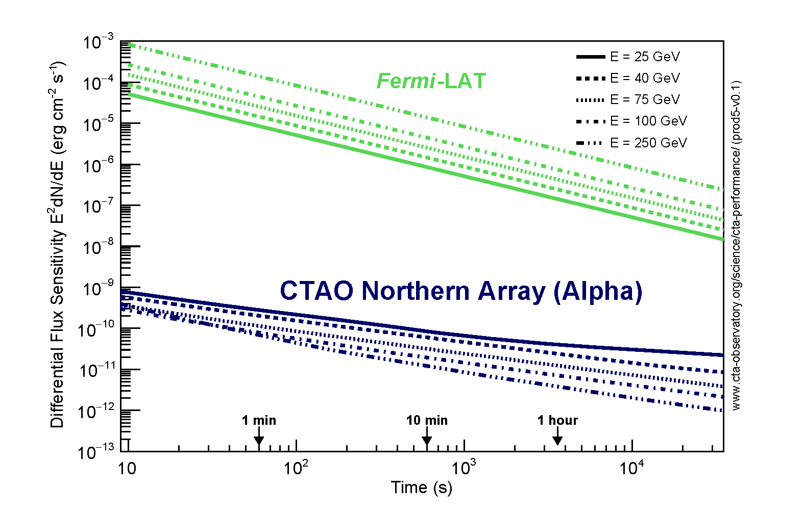
For each observation time, the sensitivity curve may either be:

• Differential flux sensitivity: E² dN/dE [GeV cm⁻² s⁻¹]
• Integral: Minimum detectable spectral flux [GeV cm⁻² s⁻¹] or photon flux [cm⁻² s⁻¹]

These curves depend on:

• Instrument Response Functions (IRFs): Define telescope performance
• Observing conditions: Zenith angle, azimuth, site (North/South)
• Energy range: Energy window of interest
• Source spectrum: The assumed spectral shape
• Region of interest: Spatial extraction region size

Creating a Sensitivity Calculator

sensipy provides the Sensitivity class for calculating sensitivity curves using Gammapy:

from sensipy.ctaoirf import IRFHouse
from sensipy.sensitivity import Sensitivity
import astropy.units as u

# Load IRFs
house = IRFHouse(base_directory="./IRFs/CTAO")
irf = house.get_irf(
    site="south",
    configuration="alpha",
    zenith=20,
    duration=1800,  # seconds
    azimuth="average",
    version="prod5-v0.1",
)

# Create sensitivity calculator
sensitivity = Sensitivity(
    irf=irf,
    observatory=f"ctao_{irf.site.name}",  # "ctao_south"
    min_energy=20 * u.GeV,
    max_energy=10 * u.TeV,
    radius=3.0 * u.deg,  # Region of interest radius
)

Key Parameters

Parameter	Description	Typical Value
irf	Instrument response function	From IRFHouse
observatory	Observatory name	"ctao_south" or "ctao_north"
min_energy	Minimum energy	20 GeV or 0.02 TeV
max_energy	Maximum energy	10 TeV
radius	Extraction region radius	3.0 deg (for point sources)
n_sensitivity_points	Number of time points	16 (default)

Computing Sensitivity for a Source

Once you have a Source object with a time-resolved spectrum, you can compute the sensitivity curve:

Basic Example

from sensipy.ctaoirf import IRFHouse
from sensipy.source import Source
from sensipy.sensitivity import Sensitivity
from sensipy.util import get_data_path
import astropy.units as u

# Load IRFs
house = IRFHouse(base_directory="./IRFs/CTAO")
irf = house.get_irf(
    site="south",
    configuration="alpha",
    zenith=20,
    duration=1800,
    azimuth="average",
    version="prod5-v0.1",
)

# Load source
mock_data_path = get_data_path("mock_data/GRB_42_mock.csv")
source = Source(
    filepath=str(mock_data_path),
    min_energy=20 * u.GeV,
    max_energy=10 * u.TeV,
    ebl="franceschini"
)

# Create sensitivity calculator
sens = Sensitivity(
    irf=irf,
    observatory="ctao_south",
    min_energy=20 * u.GeV,
    max_energy=10 * u.TeV,
    radius=3.0 * u.deg,
)

# Compute sensitivity curve for this source
sens.get_sensitivity_curve(source=source)

# Access the sensitivity curve
print(sens.sensitivity_curve)
print(sens.photon_flux_curve)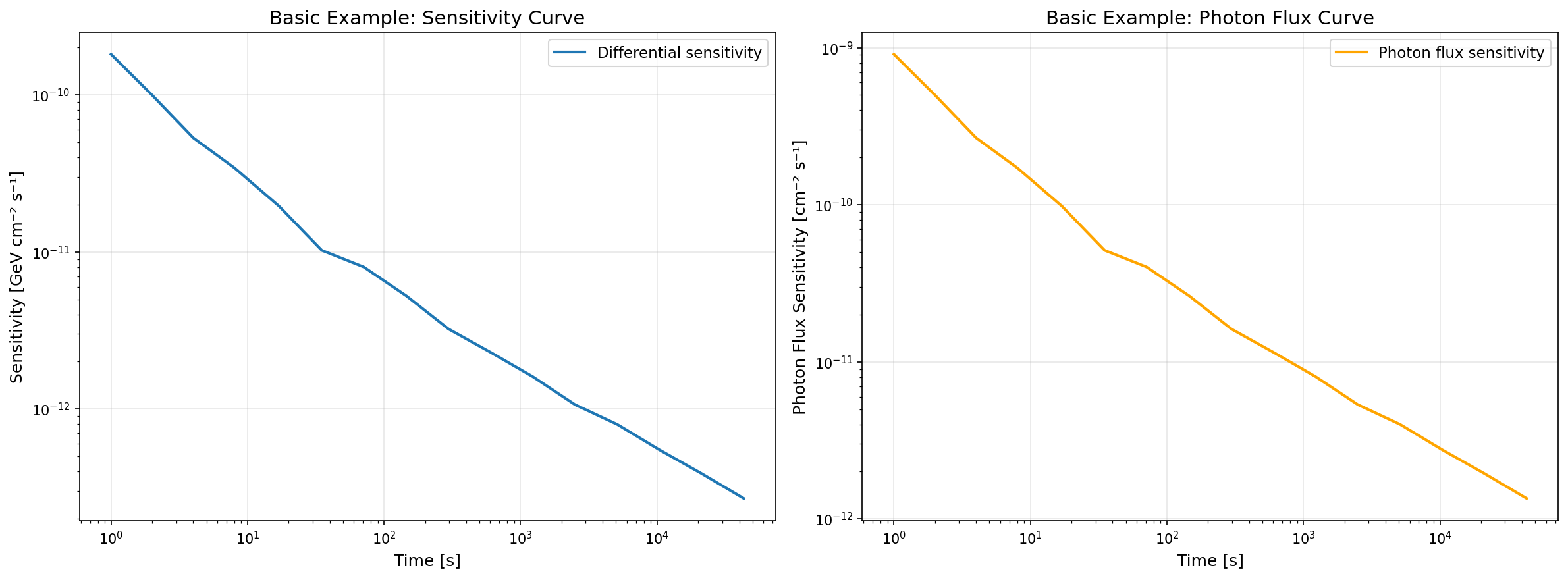

Custom Time Range

from sensipy.ctaoirf import IRFHouse
from sensipy.source import Source
from sensipy.sensitivity import Sensitivity
from sensipy.util import get_data_path
import astropy.units as u

# Load IRFs
house = IRFHouse(base_directory="./IRFs/CTAO")
irf = house.get_irf(
    site="south",
    configuration="alpha",
    zenith=20,
    duration=1800,
    azimuth="average",
    version="prod5-v0.1",
)

# Load source
mock_data_path = get_data_path("mock_data/GRB_42_mock.csv")
source = Source(
    filepath=str(mock_data_path),
    min_energy=20 * u.GeV,
    max_energy=10 * u.TeV,
    ebl="franceschini"
)

# Specify custom time range
sens = Sensitivity(
    irf=irf,
    observatory="ctao_south",
    min_energy=20 * u.GeV,
    max_energy=10 * u.TeV,
    radius=3.0 * u.deg,
    min_time=10 * u.s,       # Start at 10 seconds
    max_time=36000 * u.s,    # Up to 10 hours
    n_sensitivity_points=20,  # 20 time points
)

sens.get_sensitivity_curve(source=source)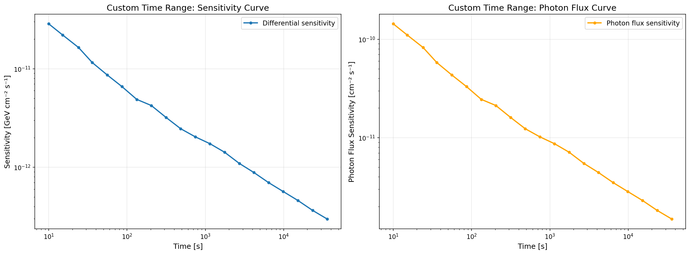

Pre-computed Curves

from sensipy.ctaoirf import IRFHouse
from sensipy.sensitivity import Sensitivity
import astropy.units as u
import numpy as np

# Load IRFs
house = IRFHouse(base_directory="./IRFs/CTAO")
irf = house.get_irf(
    site="south",
    configuration="alpha",
    zenith=20,
    duration=1800,
    azimuth="average",
    version="prod5-v0.1",
)

# Use pre-computed sensitivity values
# Note: n_sensitivity_points must match the length of the curves
sens_values = np.array([
    1.74e-10, 1.10e-10, 5.81e-11, 3.41e-11, 1.87e-11,
    1.12e-11, 7.64e-12, 4.51e-12, 2.95e-12, 2.14e-12,
    1.50e-12, 1.16e-12, 7.62e-13, 5.61e-13, 3.96e-13,
    2.71e-13, 1.85e-13, 1.27e-13, 8.70e-14, 5.95e-14
]) * u.Unit("erg / (cm2 s)")
photon_flux_values = np.array([
    8.72e-10, 5.52e-10, 2.91e-10, 1.71e-10, 9.36e-11,
    5.63e-11, 3.83e-11, 2.26e-11, 1.48e-11, 1.07e-11,
    7.52e-12, 5.83e-12, 3.82e-12, 2.81e-12, 1.98e-12,
    1.36e-12, 9.27e-13, 6.35e-13, 4.35e-13, 2.98e-13
]) * u.Unit("1 / (cm2 s)")

sens = Sensitivity(
    observatory="ctao_south",
    radius=3.0 * u.deg,
    min_energy=20 * u.GeV,
    max_energy=10 * u.TeV,
    min_time=10 * u.s,        # Match the time range of your pre-computed curves
    max_time=10000 * u.s,     # 10s to 10,000s
    n_sensitivity_points=20,   # Must match the length of your curves
    sensitivity_curve=sens_values,
    photon_flux_curve=photon_flux_values,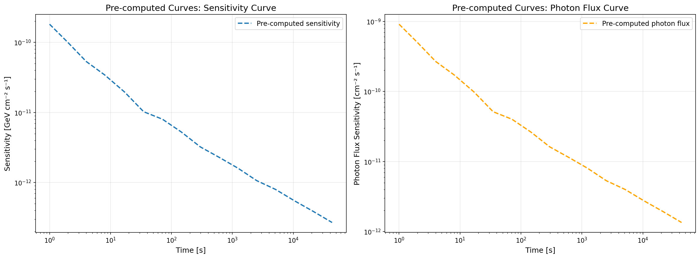
)

Querying Sensitivity Values

After computing the sensitivity curve, you can query sensitivity at arbitrary times:

from sensipy.ctaoirf import IRFHouse
from sensipy.source import Source
from sensipy.sensitivity import Sensitivity
from sensipy.util import get_data_path
import astropy.units as u

# Load IRFs
house = IRFHouse(base_directory="./IRFs/CTAO")
irf = house.get_irf(
    site="south",
    configuration="alpha",
    zenith=20,
    duration=1800,
    azimuth="average",
    version="prod5-v0.1",
)

# Load source
mock_data_path = get_data_path("mock_data/GRB_42_mock.csv")
source = Source(
    filepath=str(mock_data_path),
    min_energy=20 * u.GeV,
    max_energy=10 * u.TeV,
    ebl="franceschini"
)

# Create sensitivity calculator and compute curve
sens = Sensitivity(
    irf=irf,
    observatory="ctao_south",
    min_energy=20 * u.GeV,
    max_energy=10 * u.TeV,
    radius=3.0 * u.deg,
)
sens.get_sensitivity_curve(source=source)

# Get sensitivity at a specific time
time = 1000 * u.s
diff_sens = sens.get(time, mode="sensitivity")
phot_flux = sens.get(time, mode="photon_flux")

print(f"At t={time}:")
print(f"  Differential sensitivity: {diff_sens}")
print(f"  Photon flux sensitivity: {phot_flux}")

Sensitivity Modes

sensipy supports two sensitivity modes:

1. Differential Sensitivity

The minimum detectable energy flux per unit energy (dN/dE):

# Differential sensitivity in erg cm⁻² s⁻¹
diff_sens = sens.get(time, mode="sensitivity")

Unit: erg cm⁻² s⁻¹ or TeV cm⁻² s⁻¹

2. Photon Flux Sensitivity

The minimum detectable photon flux (integrated over energy):

# Photon flux sensitivity in cm⁻² s⁻¹
phot_flux = sens.get(time, mode="photon_flux")

Unit: cm⁻² s⁻¹

Direct Sensitivity Calculation: Integral vs Differential

sensipy provides get_sensitivity_from_model() for directly calculating sensitivity at a specific time using a spectral model. This method supports two types of sensitivity calculations:

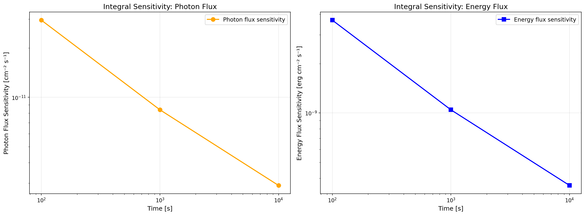
Integral Sensitivity

Integral sensitivity calculates the minimum detectable flux integrated over the entire energy range. It returns a single value representing the total photon flux or energy flux needed for detection.

Key characteristics:

• Returns a single sensitivity value for the entire energy range
• Units: Photon flux [cm⁻² s⁻¹] or Energy flux [erg cm⁻² s⁻¹]
• Uses Monte Carlo simulations with iterative root finding
• More computationally intensive but accounts for full spectral shape

from sensipy.ctaoirf import IRFHouse
from sensipy.sensitivity import Sensitivity
from gammapy.modeling.models import PowerLawSpectralModel
import astropy.units as u

# Load IRFs
house = IRFHouse(base_directory="./IRFs/CTAO")
irf = house.get_irf(
    site="south",
    configuration="alpha",
    zenith=20,
    duration=1800,
    azimuth="average",
    version="prod5-v0.1",
)

# Create a sensitivity calculator
sens = Sensitivity(
    irf=irf,
    observatory="ctao_south",
    min_energy=20 * u.GeV,
    max_energy=10 * u.TeV,
    radius=3.0 * u.deg,
)

# Define a spectral model (e.g., power law)
spectral_model = PowerLawSpectralModel(
    index=2.0,
    amplitude=1e-12 * u.Unit("cm-2 s-1 TeV-1"),
    reference=1 * u.TeV,
)

# Calculate integral sensitivity at a specific time
time = 1000 * u.s
result = sens.get_sensitivity_from_model(
    t=time,
    spectral_model=spectral_model,
    sensitivity_type="integral",
    redshift=0.0,  # Set to > 0 for extragalactic sources
)

print(f"Photon flux sensitivity: {result['photon_flux']}")
print(f"Energy flux sensitivity: {result['energy_flux']}")

Examples for a power law spectral model with index 2.0 at three different timesteps:

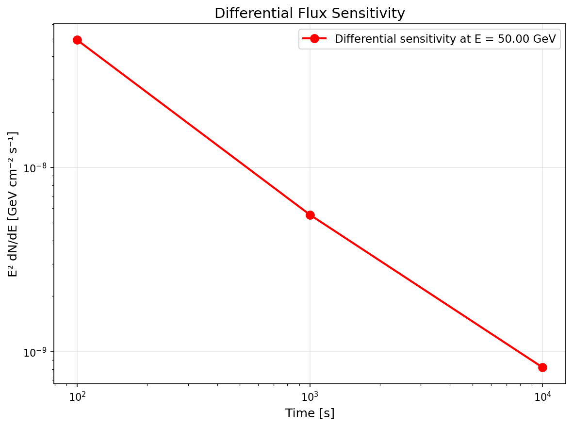
Differential Sensitivity

Differential sensitivity calculates the minimum detectable flux per unit energy at each energy bin. It returns a table with sensitivity values as a function of energy.

Key characteristics:

• Returns sensitivity values for each energy bin
• Units: dN/dE [GeV⁻¹ cm⁻² s⁻¹] at each energy
• Uses analytical background estimation
• Faster computation, provides energy-dependent sensitivity

from sensipy.ctaoirf import IRFHouse
from sensipy.sensitivity import Sensitivity
from gammapy.modeling.models import PowerLawSpectralModel
import astropy.units as u

# Load IRFs
house = IRFHouse(base_directory="./IRFs/CTAO")
irf = house.get_irf(
    site="south",
    configuration="alpha",
    zenith=20,
    duration=1800,
    azimuth="average",
    version="prod5-v0.1",
)

# Create a sensitivity calculator
sens = Sensitivity(
    irf=irf,
    observatory="ctao_south",
    min_energy=20 * u.GeV,
    max_energy=10 * u.TeV,
    radius=3.0 * u.deg,
)

# Define a spectral model
spectral_model = PowerLawSpectralModel(
    index=2.0,
    amplitude=1e-12 * u.Unit("cm-2 s-1 TeV-1"),
    reference=1 * u.TeV,
)

# Calculate differential sensitivity at a specific time
time = 1000 * u.s
result_table = sens.get_sensitivity_from_model(
    t=time,
    spectral_model=spectral_model,
    sensitivity_type="differential",
    redshift=0.0,
)

# The result is a Table with columns: energy, e_min, e_max, sensitivity
print(result_table)

Example for a power law spectral model with index 2.0 at three different timesteps:

When to Use Each Type

Use Integral Sensitivity when:

• You need a single sensitivity value for the entire energy range
• Comparing total flux requirements across different sources
• Working with sources where the full spectral shape matters
• You have computational resources for more accurate calculations

Use Differential Sensitivity when:

• You need energy-dependent sensitivity information
• Analyzing which energy ranges contribute most to detection
• Comparing sensitivity across different energy bands
• You need faster computation times

Sensitivity and Source Spectra

The sensitivity calculation uses the source spectral shape to optimize energy binning and background estimation. This is why you pass a Source object (with get_sensitivity_curve(source=source)).

Spectral Template Scaling

Internally, sensipy uses a ScaledTemplateModel to adjust the source normalization while preserving its spectral shape. This allows the code to find the minimum flux level that achieves the target significance.

from sensipy.sensitivity import ScaledTemplateModel
from gammapy.modeling.models import TemplateSpectralModel
import astropy.units as u
import numpy as np

# Create a template spectral model with energy and flux values
energy = np.logspace(-1, 2, 10) * u.TeV  # 0.1 to 100 TeV
values = np.ones(10) * u.Unit("1 / (TeV s cm2)")  # Constant flux

template_model = TemplateSpectralModel(energy=energy, values=values)

# Create a scaled template from the Gammapy model
scaled_model = ScaledTemplateModel.from_template(
    model=template_model,
    scaling_factor=1e-6  # Scale down initial normalization
)

# The scaling factor can be adjusted
scaled_model.scaling_factor = 0.5  # Reduce flux by 50%

Note

Most users don’t need to interact with ScaledTemplateModel directly - it’s used internally by the sensitivity calculator.