Detectability Analysis

Overview

The detectability module provides tools for analyzing and visualizing source detectability data from lookup tables. It allows you to filter data, calculate detectability statistics, and create publication-quality heatmaps showing the fraction of sources detected at various delay times and observation times.

Key Features

• Flexible data loading: Works with Parquet or CSV files
• Custom column names: Supports any column naming convention
• Powerful filtering: Filter by any column using flexible operators
• Customizable visualization: Create heatmaps with full control over appearance
• Grid plotting: Compare multiple configurations side-by-side

Basic Usage

Loading Data

The LookupData class is the main interface for working with detectability data:

from sensipy.detectability import LookupData
from sensipy.data.create_mock_lookup import create_mock_lookup_table
from pathlib import Path
import tempfile

# Create a mock lookup table for demonstration
with tempfile.TemporaryDirectory() as tmpdir:
    lookup_path = create_mock_lookup_table(
        event_ids=[1, 2, 3, 4, 5],
        sites=["north", "south"],
        zeniths=[20, 40, 60],
        delays=[10, 30, 100, 300, 1000, 3000, 10000],
        output_dir=tmpdir,
    )

    # Load the data
    data = LookupData(lookup_path)
    print(f"Loaded {len(data)} rows")

Filtering Data

Filter data by any column using flexible operators:

# Filter by site and zenith
data.set_filters(
    ("irf_site", "==", "north"),
    ("irf_zenith", "<", 40),
)

# Filter by event IDs
data.set_filters(("event_id", "in", [1, 2, 3]))

# Multiple filters can be combined
data.set_filters(
    ("irf_site", "==", "south"),
    ("irf_zenith", "==", 20),
    ("event_id", ">=", 2),
)

Supported operators: ==, =, <, >, <=, >=, in, not in, notin

Creating Heatmaps

Generate detectability heatmaps with customizable options:

import matplotlib.pyplot as plt

# Set observation times for the analysis
data.set_observation_times(np.logspace(1, np.log10(3600), 10, dtype=int))

# Create a basic heatmap
fig, ax = plt.subplots(figsize=(10, 8))
data.plot(
    ax=ax,
    title="Source Detectability: CTAO North, z20",
    max_exposure=1,  # Maximum exposure time in hours
    return_ax=True,
)
plt.tight_layout()
plt.savefig("detectability_plot.png", dpi=150, bbox_inches="tight")
plt.close()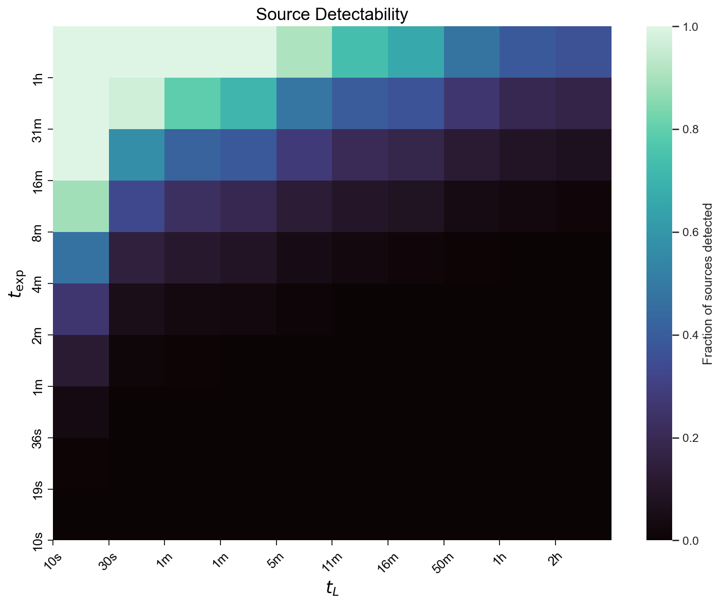

Customizing Plots

The plot() method offers extensive customization options:

data.plot(
    ax=ax,
    title="Custom Detectability Plot",
    max_exposure=2,  # Maximum exposure time in hours
    as_percent=True,  # Display as percentages (0-100)
    color_scheme="viridis",  # Colormap name
    color_scale="log",  # Logarithmic color scale
    min_value=0.1,  # Minimum value for color scale
    max_value=0.8,  # Maximum value for color scale
    n_labels=15,  # Number of tick labels
    tick_fontsize=10,  # Font size for tick labels
    label_fontsize=14,  # Font size for axis labels
    square=False,  # Non-square cells
    annotate=True,  # Annotate cells with values
)

Custom Title Generation

You can provide a custom title string or use a callback function:

# Using a string title
data.plot(title="My Custom Title")

# Using a callback function
def title_callback(data_df, results_df):
    n_total = results_df.groupby("delay").total.first().iloc[0]
    return f"Detectability Analysis (n={n_total} sources)"

data.plot(title_callback=title_callback)

Working with Custom Column Names

If your lookup table uses different column names, specify them when creating the LookupData object:

# Table with custom column names
data = LookupData(
    "my_lookup_table.parquet",
    delay_column="delay_col",  # Custom delay column name
    obs_time_column="time_col",  # Custom observation time column name
)

# Filtering and plotting work the same way
data.set_filters(("event_id", "==", 1))
data.plot(title="Custom Columns Example")

Advanced Examples

Filtered Analysis

Analyze detectability for specific subsets of your data:

# Filter for south site, low zenith, specific events
data.set_filters(
    ("irf_site", "==", "south"),
    ("irf_zenith", "<=", 40),
)

data.set_observation_times(np.logspace(1, np.log10(7200), 10, dtype=int))

fig, ax = plt.subplots(figsize=(10, 8))
data.plot(
    ax=ax,
    title="Detectability: South Site, Low Zenith, Events 1-3",
    max_exposure=2,
    as_percent=True,
    color_scheme="viridis",
    return_ax=True,
)
plt.tight_layout()
plt.savefig("filtered_detectability.png", dpi=150, bbox_inches="tight")
plt.close()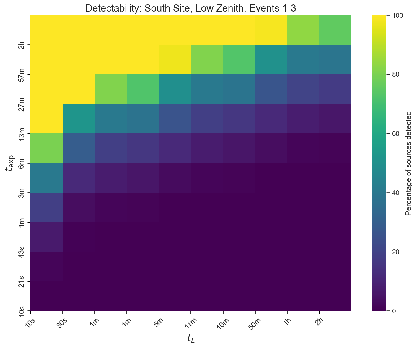

Grid of Heatmaps

Compare multiple configurations side-by-side using create_heatmap_grid():

from sensipy.detectability import create_heatmap_grid

# Create multiple LookupData objects with different filters
data_north_z20 = LookupData(lookup_path)
data_north_z20.set_filters(("irf_site", "==", "north"), ("irf_zenith", "==", 20))

data_north_z40 = LookupData(lookup_path)
data_north_z40.set_filters(("irf_site", "==", "north"), ("irf_zenith", "==", 40))

data_south_z20 = LookupData(lookup_path)
data_south_z20.set_filters(("irf_site", "==", "south"), ("irf_zenith", "==", 20))

data_south_z40 = LookupData(lookup_path)
data_south_z40.set_filters(("irf_site", "==", "south"), ("irf_zenith", "==", 40))

# Create a 2x2 grid
fig, axes = create_heatmap_grid(
    [data_north_z20, data_north_z40, data_south_z20, data_south_z40],
    grid_size=(2, 2),
    max_exposure=1,
    title="Detectability Comparison: Site and Zenith Configurations",
    subtitles=[
        "North, z20",
        "North, z40",
        "South, z20",
        "South, z40",
    ],
    cmap="mako",
)
plt.savefig("detectability_grid.png", dpi=150, bbox_inches="tight")
plt.close()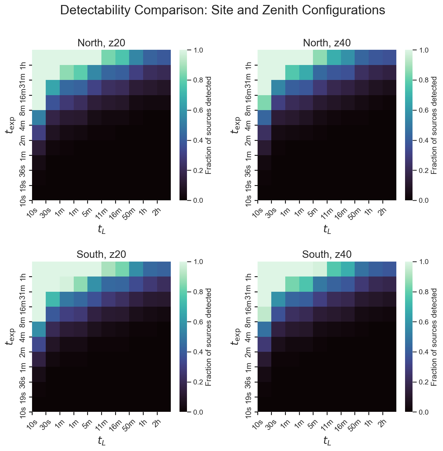

Accessing Results Data

You can access the calculated detectability results programmatically:

# Calculate results
data.set_observation_times([10, 100, 1000, 10000])
results = data.results

print(results.columns)
# ['delay', 'obs_time', 'n_seen', 'total', 'percent_seen']

# Filter results for specific delay
delay_1000 = results[results["delay"] == 1000]
print(delay_1000[["obs_time", "percent_seen"]])

Resetting Filters

Reset filters to return to the full dataset:

# Apply filters
data.set_filters(("irf_site", "==", "north"))

# Reset to full dataset
data.reset()

Data Requirements

Your lookup table must contain at least two columns:

• Delay column (default: obs_delay): Observation delay times in seconds
• Observation time column (default: obs_time): Required observation times in seconds (negative values indicate non-detection)

Additional metadata columns are optional but useful for filtering:

• event_id: Event identifier
• irf_site: Observatory site ("north" or "south")
• irf_zenith: Zenith angle in degrees
• irf_ebl_model: EBL model name
• Any other columns you want to filter by

API Reference

• See the API reference for complete function documentation